ASTM A106 Grade B Carbon Steel Pipe’s Thermal Fluid Dynamics
The case study involves the complete analysis through computational fluid dynamics. The case study is based on using ANSYS CFX software: Geometric building using ANSYS workbench, meshing the geometry through ICEM CFD, setting boundary conditions through CFX12 PRE, simulation through ANSYS CFX 12 solver and post solution through ANSYS CFX 12 post processor. The cold air on A106 Grade B Carbon Steel Pipe is actually tilted and the hot air is coming from the horizontal big diameter A106 Grade B Carbon Steel Pipe.
The result that is obtained through the above process is actually the point of explanation and focus of this study. Further the learning concepts about ANSYS meshing techniques and equations are also discussed in the introductory section of the study.
What Is CFD: Computational fluid dynamics is an application of computer aided analysis for analyzing fluids and their properties. It utilizes different approaches of algorithms and fluid mechanics formulae for the same purpose. There is different software like ANSYS which supports the feature of fluid mechanics so that a fluid interaction with the surfaces and given boundary conditions can be easily simulated and predicted in the analysis phase of a design. There are different equations like Navier Equation, RANS equation and different meshing techniques like finite difference and finite volume that are used in CFD for fluid analysis. Other meshing schemes are also there like FEM and BEM but they are not used for fluid analysis.
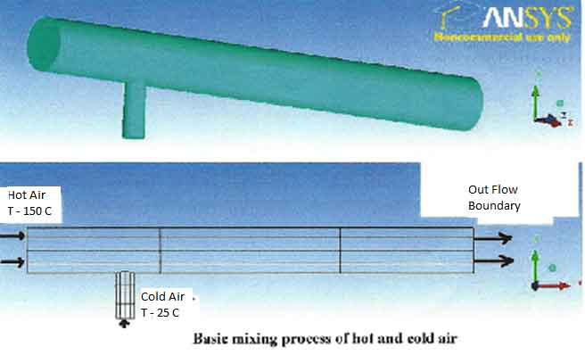
The Case Study: The study is about a case study on the same topic of computational fluid dynamics. It is actually about a basic mixing of hot gas and cold gas at temperature 150 Centigrade and 25 Centigrade respectively. The mixing is done in a A106 Grade B Carbon Steel Pipe of 500 mm length, the hot gas enters in 100 mm diameter and the cold gas enters from 20 mm diameter of other A106 Grade B Carbon Steel Pipe mounted on the main A106 Grade B Carbon Steel Pipe. The length of this A106 Grade B Carbon Steel Pipe is about 50 mm. A complete analysis of CFD has to be applied.
Methodization of the Problem Set-Up
Navier- Equations: The flow behavior in terms of velocity field for a non-turbulent, Newtonian fluid is governed by the Navier-Stokes equations. These equations are valid only for the moving flow as it describes the flow field. The Navier-Stokes equations are obtained by combining the fluid kinematics and constitutive relation into the fluid equation of motion, and eliminating some higher order tensors. Navier-stroke equation is applicable for any laminar or transient and non-viscous flow passing through passage of any geometry.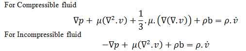
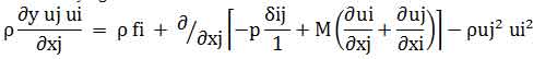
RANS: Reynolds-averaged Navier-Stokes (RANS) equations are the oldest methodology to model turbulent flow. For the turbulent flow it introduces an additional apparent stresses called Reynolds stresses. These equations are timed-average equations but are equally valid for the flows with a time-varying mean flow.
Finite Difference: Finite difference method is a commonly applicable discretization method for the solution of ordinary and partial differential equations. In this method all derivatives are exchanged by approximations that involve solution values only, so overall differential equation is reduced to a system of nonlinear equations or linear algebraic equations.
Generally;
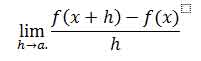
If h has a fixed but non-zero value say “a”, instead of approaching zero, this quotient is called a finite difference
Finite Volume Method: It is a 3d method of finite difference method specially designed for fluid analysis in 3d space. First of all the given domain is distributed in to numerous finite control volumes and the concerned variable is placed into the control volume’s centroid. The other stage is to integrate partial differential equations of control volume. The equation obtained by the process of integration is called discretization equation. This method reformulates the prevailing equations of partial difference in a conventional approach or in algebraic approach.
Turbulence Modeling: Turbulence modeling is a technique of modeling that is used to analyze and foresee the effects of chaotic movement like turbulence in some model space. The chief purpose of this technique of modeling is to acquire a model of analysis in which velocity and other factors of turbulence can be incorporated. The additional stresses caused by the chaotic movement of fluids are modeled by eddy viscosity. Here viscosity can be shown as:
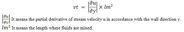
k-ε model : K-Ε MODEL is the most common and essential method for turbulence modeling. It is also known as two equation models because it utilized two equations for the solution.
The mean flow is given by;
Problem Definition: Brief Description to ANSYS CFX CODE:
Geometry: The geometry of the problem is very simple. It is a horizontal A106 Grade B Carbon Steel Pipe whose one end is closed and is fed by a narrow passage from the bottom. Using ANSYS Workbench 12 geometry generation feather it can easily be formed by using feather approach like extruding a circular section of required diameters for the flow passages (horizontal and vertical). User can also create geometry into some CAD software (e.g. Pro-e) which is compatible with ANSYS to import.
Mesh: Since this is a CFX problem that needs more accuracy, poor meshing can greatly distracts the results. For the fluid element it is suggested that ANSYS Workbench auto-meshing feather should be used. By defining variable density mesh (two extreme limits for the element size) we can get a great control our accuracy of solution with the shortest computational time. The element type that results by auto meshing option basically generates tetrahedral elements at the middle sections of the control volume and hexahedral or prism element at the surfaces of the system. Also mesh concentration is more in the areas where the flow behavior is critical and usually rough meshing is carried out to get remarkably accurate results with short processing duration.
Boundary Conditions:
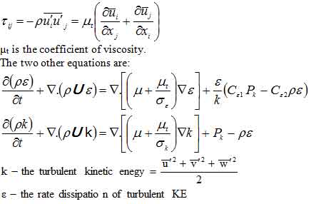
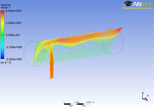
Boundary Condition for Velocity Profile: Reference to the figure “Velocity Vector-1” it can easily be stated that boundary conditions for the velocity field are;
6 m/s @ Section-1 (from where the flow is entering into the system
0 m/s @ Section-2 (closed end of the system)
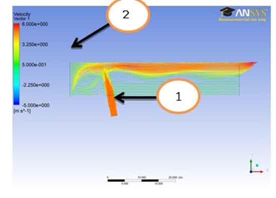
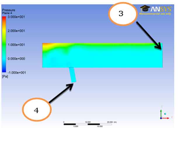
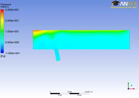
Boundary Condition for Pressure Profile: For pressure reference to the figure “Pressure Plane -4” it can easily be stated that boundary conditions for the pressure field are;
0 Pa. (Gauge) @ Section-3 & Section-4read out from the result (It is seemed that both outlets are open to atmosphere)
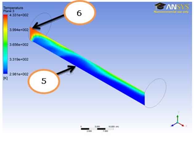
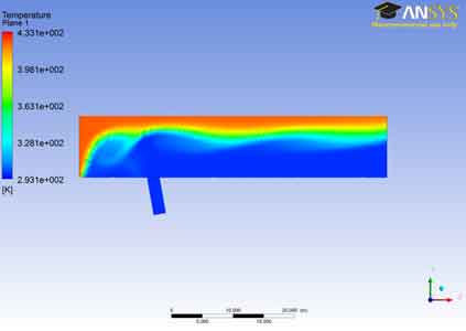
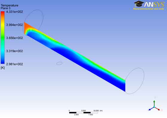
Boundary Condition for Temperature Profile: For temperature, from the figure “Temperature Plane -3” we can state the boundary conditions for the temperature field;
433 K @ Section-6 read out from the result (it is seemed that close end is maintained at that temperature.
298 K @ Section-5 read out from the result (the fluid injected through the section is at ambient temperature of 298 K
Solver: For the solver the iterations for the refinement of the result should be defined, also for the case of transient and turbulent analysis with temperature field involved time domain must be specified.
Results Discussions:
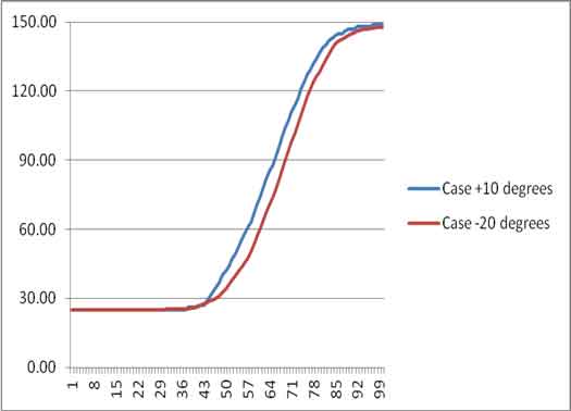
Comparison Of Two Profiles 10 And 20 Degrees Of Temperature: As one can see analysing the tables of temperature by the change of angle, the result of two cases are initially same. Nearly about 1 to 40 of y in mm the temperature difference of the fluids in the two cases are not much. At 1 mm case 10 degree’s temperature is 25 Centigrade while case 20 degree’s temperature is 25.175 Centigrade. Till 40 mm the case 10 degrees has 26 Centigrade while the case 20 degree has 25.859. Now as we go onwards the temperature difference is increasing. Temperature of fluid with 10 degree tilt is more throughout than the other profile of 20 degree tilt. At 100 mm we can see that 10 degree tilt has 149 Centigrade and 20 degree tilt has 147.7 Centigrade. The Y axis shows the temperature line and the X axis shows the displacement in Y direction of the profile.
Velocity Field: Contours: The velocity vector-1 represents the velocity field the fluid is injected through the bottom passage therefore the lower left of the figure represents region of higher velocity similarly because of the fact that the left half of the horizontal passage is closed the flow form a vortex showed by the upper left half of the system. The remaining flow is then directed toward the right. One can also observed that the fluid entered into the system is not same as the fluid prevailed inside the system which is obvious from the fact that the flow entered the horizontal passage is positioned at the top throughout.
The Velocity vector 1 shows that the velocity at the outer region is near to the maximum value ranging from 3.25e+000 to 6.000e+000. The reason for this might be due to the turbulency of the fluid. As the fluid flow changes from laminar to turbulent the velocity increases and so as the disturbance increases between the layers of the fluids. There are two figures for vector 1 both showing the same results.
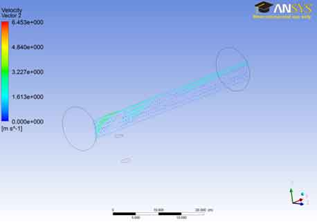
The velocity vector 2 shows that the velocity of the fluid in the lower region remains lower and steady. The flow is steady during this portion and it is laminar. The disturbances are minimum between the adjacent layers and as a result there is lesser temperature gradients and lesser pressures in this area. This is the desirable condition but as the fluid we move towards the outer region the velocities tend to increase and so as the turbulence..
Pressure Field: Contours : From the analysis of the pressure plane 4 we can see that the pressure remains near zero value during most of the part of the A106 Grade B Carbon Steel Pipe and as we go from the bottom to the outer part of plane 4 ,the pressure increases gradually from 0 to about 2.00 e+001.The pressure of the fluid in the A106 Grade B Carbon Steel Pipe is kept near to zero or negative for most of the area inside the A106 Grade B Carbon Steel Pipe so that the pressure around the A106 Grade B Carbon Steel Pipe ( atmospheric pressure) remains greater and the oil(fluid inside the pipe) does not burst the A106 Grade B Carbon Steel Pipe . Pipelines commonly have areas of negative pressure. Usually this is an intentional choice. For example, undersea pipelines used for oil and other materials are kept in a state of negative pressure so that if they rupture, seawater will flood the A106 Grade B Carbon Steel Pipe. If the pipes were positively pressurized, their contents would explode into the ocean, potentially creating a hazardous spill.
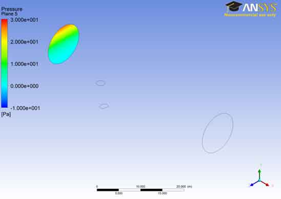
We can see that at plane 5 the pressure of the fluid remains near to zero value for most of the cross-sectional area. As we go in the outer region the pressure raises up to the value of 3.00 e+001.This is similar to the interpretation for the previous case. Different colors in the area shows the variation of pressure in the A106 Grade B Carbon Steel Pipe ranging from blue being the least to red which is the highest.
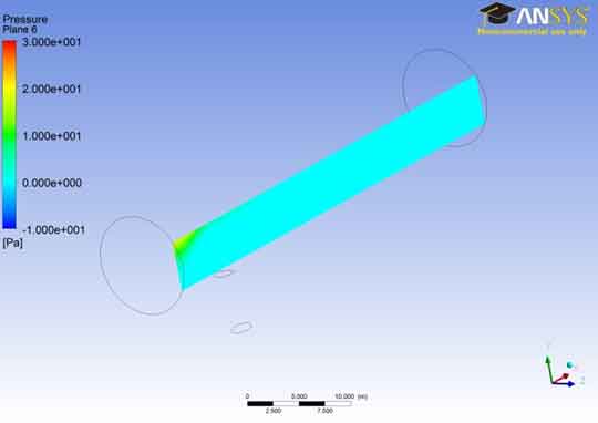
In the pressure contour for plane 6, the results are similar to that of the last two planes. The pressure remains near to zero value for most of the area of the A106 Grade B Carbon Steel Pipe as indicated in the last two cases. The reason to keep this pressure was explained in the first case. It is noted that the pressure increases as the fluid reaches near the boundary of the A106 Grade B Carbon Steel Pipe and collides with it.
Temperature Field: Contours: The temperature contour for plane 1 shows that the stream entering from the left of the A106 Grade B Carbon Steel Pipe inlet has more hot temperature region at the inlet. But as soon as it goes forward the cold stream of air has reduced its location to the top of the A106 Grade B Carbon Steel Pipe.
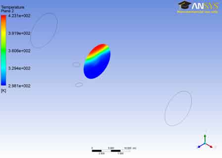
The temperature contour for plane 2 i.e. in the middle of the A106 Grade B Carbon Steel Pipe is shown in the figure. We can see that the temperature at the lower end of the A106 Grade B Carbon Steel Pipe is lowest and remains at this lowest value for most of the part of the A106 Grade B Carbon Steel Pipe. The temperature increases as the fluid moves away from the bottom surface. The temperature is maximum at the outer end of the A106 Grade B Carbon Steel Pipe. This might be due to the decreased heat transfer rate at the outer end due to the insulation that is applied at the outer end.
In the temperature contour for plane 3 one can see that the temperature remains near 2.981e+002 for the most part. The temperature gradually rises and reaches a maximum value i.e. 4.33e+002.The rise of temperature also shows that the flows becomes turbulent and generation of eddies has taken place. The turbulence increases as the fluid flows near the outer region so the temperature has risen as well.
Vectors: The Velocity vector 1 shows that the velocity at the outer region is near to the maximum value ranging from 3.25e+000 to 6.000e+000. The reason for this might be due to the turbulency of the fluid. As the fluid flow changes from laminar to turbulent the velocity increases and so as the disturbance increases between the layers of the fluids. There are two figures for vector 1 both showing the same results.
The velocity vector 2 shows that the velocity of the fluid in the lower region remains lower and steady. The flow is steady during this portion and it is laminar. The disturbances are minimum between the adjacent layers and as a result there is lesser temperature gradients and lesser pressures in this area. This is the desirable condition but as the fluid we move towards the outer region the velocities tend to increase and so as the turbulency.
CONCLUSION: In this case study, several different analyses were performed. The study initiated with the introduction of computational fluid dynamics, where the case object was also discussed. Then for the problem set up we analyzed different equations that will be used by the software for the analysis of the given case. This includes Navier equations, RANS in which the two different meshing techniques are also discussed. Then discussion started on turbulence modeling. Then we came across with the stage of Ansys CFX code where geometry of the given object, meshing boundary condition and solution were discussed. Then after the processing the software the results were discussed.
- The two profiles of 10 degree tilt and 20 degree tilt was discussed with respect to temperature difference, hence through CFD based analyses of images in this document about a flow analysis, flow through a horizontal A106 Grade B Carbon Steel Pipe fed by a passage from the bottom and through side hole, we have come to the following conclusions:
- The pressure inside the A106 Grade B Carbon Steel Pipe remains to the zero value for most of the part due to the reason that the pressure is always kept below the atmospheric pressure so that the fluid doesn’t burst the A106 Grade B Carbon Steel Pipe.
- Temperatures have remained steady and low for the lower part of the A106 Grade B Carbon Steel Pipe but as we go near the upper region the temperature rises due to turbulence.
- Velocities of the particles have also been uniform and low during the laminar flow but as the flow becomes disturbed the velocities have increased which can be seen in velocity vector 1.
REFERENCES:
Anderson, John D. Computational Fluid Dynamics: The Basics With Applications. McGraw-Hill Science, 1995.
Shah, Tasneem M. and Zafar U. Koreshi Sadaf Siddiq. An analysis and comparison of tube natural frequency modes with fluctuating force frequency from the thermal cross-flow fluid in 300 MWe PWR. International Journal of Engineering and Technology , n.d.
Tannehill, John. Computational Fluid mechanics and Heat Transfer. Taylor and Francis, 1997.
Toro, E. F. Riemann Solvers and Numerical Methods for Fluid Dynamics. Springer-Verlag, 1999.
Wesseling, Pieter. Principles of Computational Fluid Dynamics. Springer-Verlag, 2001.